Smith-Waterman dynamics programming for calculating edit distance

In Edit Distance Calculation - Recursive Edit Distance of Prefixes between 2 string X and Y, we discussed that the key is to break the problem down to smaller subproblems - shorten X and/or Y by one character at a time, until either X or Y becomes an empty string.

The recursive process to solve smaller problems (shorter strings) of edit distances can be summarized as follows:

$$\begin{gathered} \begin{array}{c}edit\_dist(X,Y)=min\{\begin{array}{l}edit\_dist(\alpha ,\beta )+\delta (x,y)\\ edit\_dist(\alpha x,\beta )+1\\ edit\_dist(\alpha ,\beta y)+1\end{array}\end{array} \\ \text{where α and β are prefix (1 character shorter) of X and Y,} \\ \text{i.e., α = X[:-1], x = X[-1]; β = Y[:-1]; y = Y[-1]} \end{gathered}$$

Implementation in python:

def edDistRecursive(a, b): 
	if len(a) == 0: return len(b) 
	if len(b) == 0: return len(a) 
	
	delt = 1 if a[-1] != b[-1] else 0 
	
	return min(edDistRecursive(a[:-1], b[:-1]) + delt, edDistRecursive(a[:-1], b) + 1, edDistRecursive(a, b[:-1]) + 1)

The recursive method is straightforward but really slow, and the reason is the method will be calling the same subproblems many times.

As illustrated below, when comparing “ABC” with “BBC”, the recursive program will keep branching to 3 subproblems, and on the second layer of the tree, we can already see the problem of edDistRecursive("AB", "BB") being called twice.

A more specific example: if we calculate the edit distance of “Shakespeare” and “shake spear” with the recursive program, and count the number of times the subproblem of edit distance of “Shake” and “shake” is calculated (with the python code below) - the result is 8989 times!

# for edDistRecursive("Shakespear", "shake spear")
# check the number of times edDistRecursive("Shake", "shake")
# is called
n = 0
def edDistRecursive(a, b): 
  # count the time the program calcualtes the edit distance of
  # prefixes of "Shake" and "shake"
  global n
  if a == "Shake" and b == "shake":
    n += 1
  # old part of recursive function
  if len(a) == 0: return len(b) 
  if len(b) == 0: return len(a) 
	
  delt = 1 if a[-1] != b[-1] else 0 
  
  return min(edDistRecursive(a[:-1], b[:-1]) + delt, 
             edDistRecursive(a[:-1], b) + 1, 
             edDistRecursive(a, b[:-1]) + 1)
 
print(edDistRecursive("Shakespeare", "shake spear"))
print(n)

Yikes, apart from really hard to read, the recursive function wastes a lot of time repeating the same work.

A clever way to improve the algorithm is to write down the answer of each smaller problem the first time we encounter and calculate it, then resue it later instead of calculating again. This strategy of writing down or remebering the answers for resusing later is called dynamic programming.

In our problem of calculating the edit distance, the dyanmic programming strategy can be visualized as a matrix.

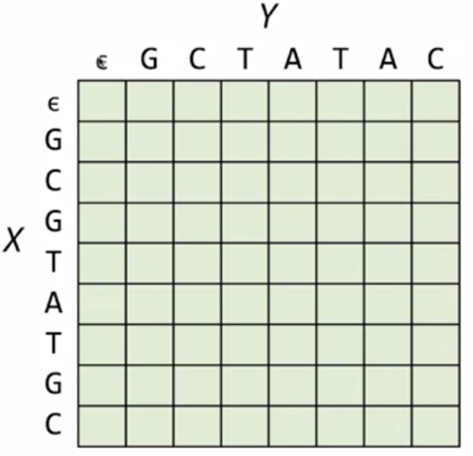
Consider X=GCGTATGC, Y=GCTATAC, we arrange a martix where each row corresponds to each character in X, and each column corresponds to each character in Y, with an extra row and column $ϵ$ represtenting the empty string.

This matrix will record the answer of edit distances of the substrings, where each elemnt at (row = n, col = m) recording the edit distance of prefix X[:m] and Y[:n].

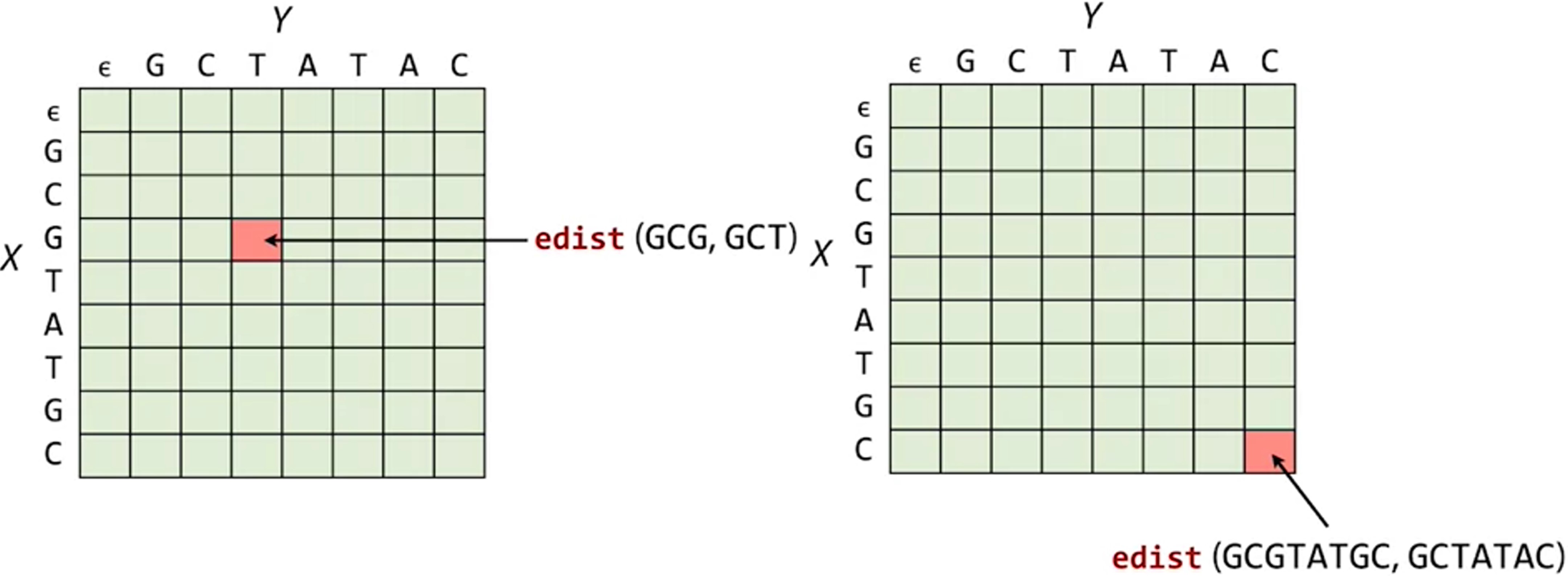
For example, the elememnt at the 4th row (n=3 for the 0-based index in python) and the 4th col (m=3) records the edit distance of X[:3] and Y[:3], which are GCG and GCT, respcectively. (The indices might be confusing due to the extra column and row representing the empty string and the first row/col has index 0, but it shouldn’t be that hard to sort out.)

The element at the lower left corner is the final answer to our question - the edit distance of X and Y.

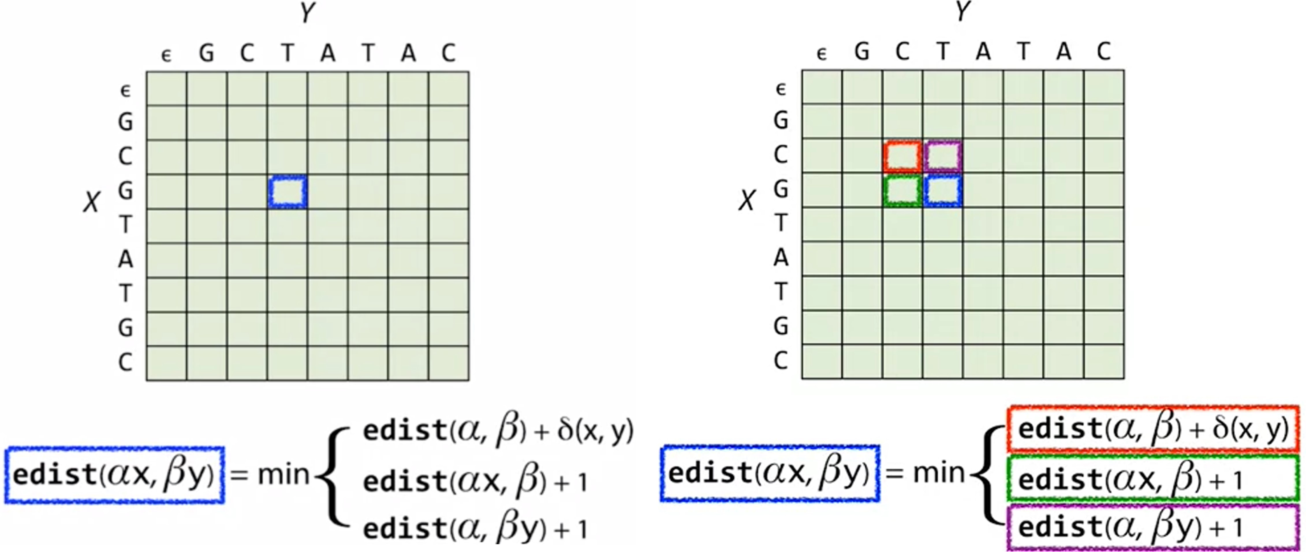
For a particular position, say the previous case of prefix GCG and GCT (m = 3; n = 3), indicated by the blue box below. To get the edit distance of the blue box, we need the edit distance of (GC, CG) - ($\alpha$, $\beta$), (GCG, GC) - ($\alpha x$, $\beta$) and (GC, GCT) - ($\alpha$, $\beta y$). Those 3 cases correspond to the box to the upper left of the blue box (the red box), the box right next to the blue box (the green box), and the box right above (the purple box).

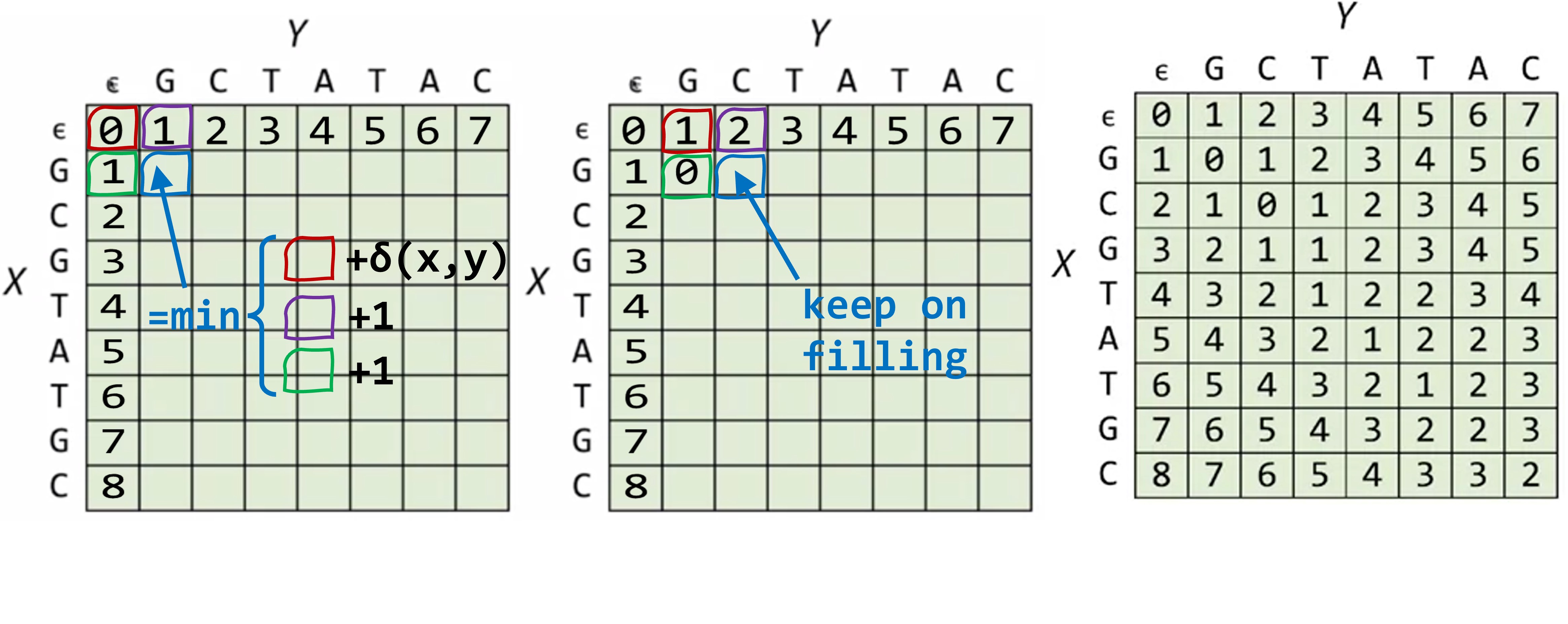
So to fill up the entire matrix and get to the answer at the lower right corner, we start by filling out the first row and first column, where the answer of the edit distance of any prefix to an empty string is obvious (it’s the length of the prefix). Then the second row can be filled one by one, since we only need the 3 boxes (upper left, left, above) to get to each box.

This clever workaround calculate each subproblem exactly once, instead of the 9000 times in the simple example shown before, which makes it a lot faster!

The matrix filling dynamic programming method was brought up by Temple F. Smith and Michael S. Waterman in 1981 in their paper “Identification of Common Molecular Subsequences” in the Journal of Molecular Biology, hence refered to as the Smith-Waterman algorithm. It is one of the most widely used algorithms in sequence alignment.